Methods
This section provides an overview of the general process and methods used to develop the UESI framework and selection of indicators. Specific details regarding the calculation of indicators are included in each individual issue chapter.
As of January 2023, the UESI includes 283 cities and almost 14,000 thousand districts, comprising cities from all continents, except Antarctica, and from multiple levels of development.
The UESI Framework
The Index includes five categories of environmental concerns: Air Quality, Climate Change, Water and Sanitation, Urban Ecosystem, and Transportation (Figure 1). Each city is gauged on environmental performance indicators within these issues as well as how different demographic group (e.g., by income and sensitive populations) are affected. For instance, neighborhoods within each city receive scores for the amount of urban tree cover canopy as well as how equitable the access to the green space is. All data are made open and available through an online portal, which provides an interactive dashboard for citizens, policymakers, and urban managers to explore in more detail where they perform well and which areas may require greater attention.

Figure 1. Categories of environmental issues and indicators assessed in the Urban Environment and Social Inclusion Index (UESI).
Data Sources
One of the key challenges in developing data for the UESI is to find an appropriate balance of spatial disaggregation, geographical and temporal availability, and quality to create a set of indicators and indices to represent the environmental performance and the equitable distribution of its benefits to cities in both hemispheres. In this sense, the datasets used for the UESI are reviewed and verified for these criteria as part of each iteration and the sources are updated accordingly to incorporate the most recent available information for each city, as well as including additional cities in the dataset, particularly from developing countries.
Unlike nationally-derived datasets, spatially explicit information at sub-urban level is generated with much less consistency. To overcome this limitation, the UESI uses primary and secondary data primarily from large-scale remote sensing datasets and open-source geospatial data, such as OpenStreetMap, which is integrated with official administrative data on population and income collected at the neighborhood and block-level. The UESI applies a set of criteria to determine which datasets to select for inclusion (see Box 1: Guiding Principles for Indicator Selection in the UESI).
All sources of data are publicly available and include:
- Satellite data from LANDSAT and MODIS products;
- Geospatial datasets, such as gridded global population, Annual Ground-Level NO2, and Gross Domestic Product;
- Open Source Transportation data and geographical boundaries from Open Street Maps;
- Official statistics on population and income from national and local governments collected through census or other initiatives.
Data Quality Tiers
For the socioeconomic variables, we prioritized the use of official population and income data from national, regional or local authorities, but for many cities, we were unable to obtain this data either because it is not readily available from official websites, or because the data does not exist (i.e. many countries and cities don’t measure or openly report income as a continuous variable but as part of other variables such as socioeconomic status or poverty status). To overcome this problem, primarily for the Equity calculations, we use a proxy for neighborhood-level income data, which is the Gross Domestic Product (GDP) data from a globally generated dataset (Kummu et. al. 2018). While not equivalent to income per capita data, we consider it the best available proxy. For the sake of transparency, the UESI classifies cities as Tier I (i.e. cities that have income per capita data available) and Tier II (i.e. cities where we use GDP per capita) to designate potential differences when comparing these cities’ equity indicators, considering that Tier II cities might have different results on the equity indicators if GDP distribution is in reality not similar to the income distribution. We encourage Tier II cities to get in touch with us with their neighborhood-level income per capita data if it is available.
Box 1: Guiding Principles for Indicator Selection in the UESI
1) Spatially-explicit
The index incorporates spatially-explicit indicators as much as possible given data availability. Because people do not experience cities uni-dimensionally, the UESI aims to incorporate spatial data as much as possible to examine patterns, trends, and differences in environmental performance throughout and between urban areas. Spatially-explicit indicators also expose variation within cities. For example, land surface temperature has been connected to population density, although this relationship is varied between cities. Identifying these differences can help urban environmental managers identify distributional impacts of various environmental policies. By combining spatially-explicit environmental and socioeconomic data, the UESI features indicators that allow us to assess how different communities are affected by environmental hazards and benefits.
2) Incorporate equity
We adopt equity and social justice as applicable end goals for our measurement framework and indicators, meaning we strive for our tools and analysis to shed light on socioeconomic drivers, patterns, and differences that can lead to disproportionate levels of environmental quality and performance. Exposing these differences requires detailed spatial data and we will continue seeking data and examples to determine how each city fares in terms of equity. In this sense, the commitment to equity echoes point 1 above.
3) Build on and support SDG 11 and other global goals
SDG 11 sets a goal to make cities “inclusive, safe, resilient, and sustainable,” which informs the design of our indicator framework as well as the selection of indicators. Because we aim for this tool to be useful for policymakers to track progress towards SDG 11 and other international policy goals, we have aligned our indicators and framework as much as possible.
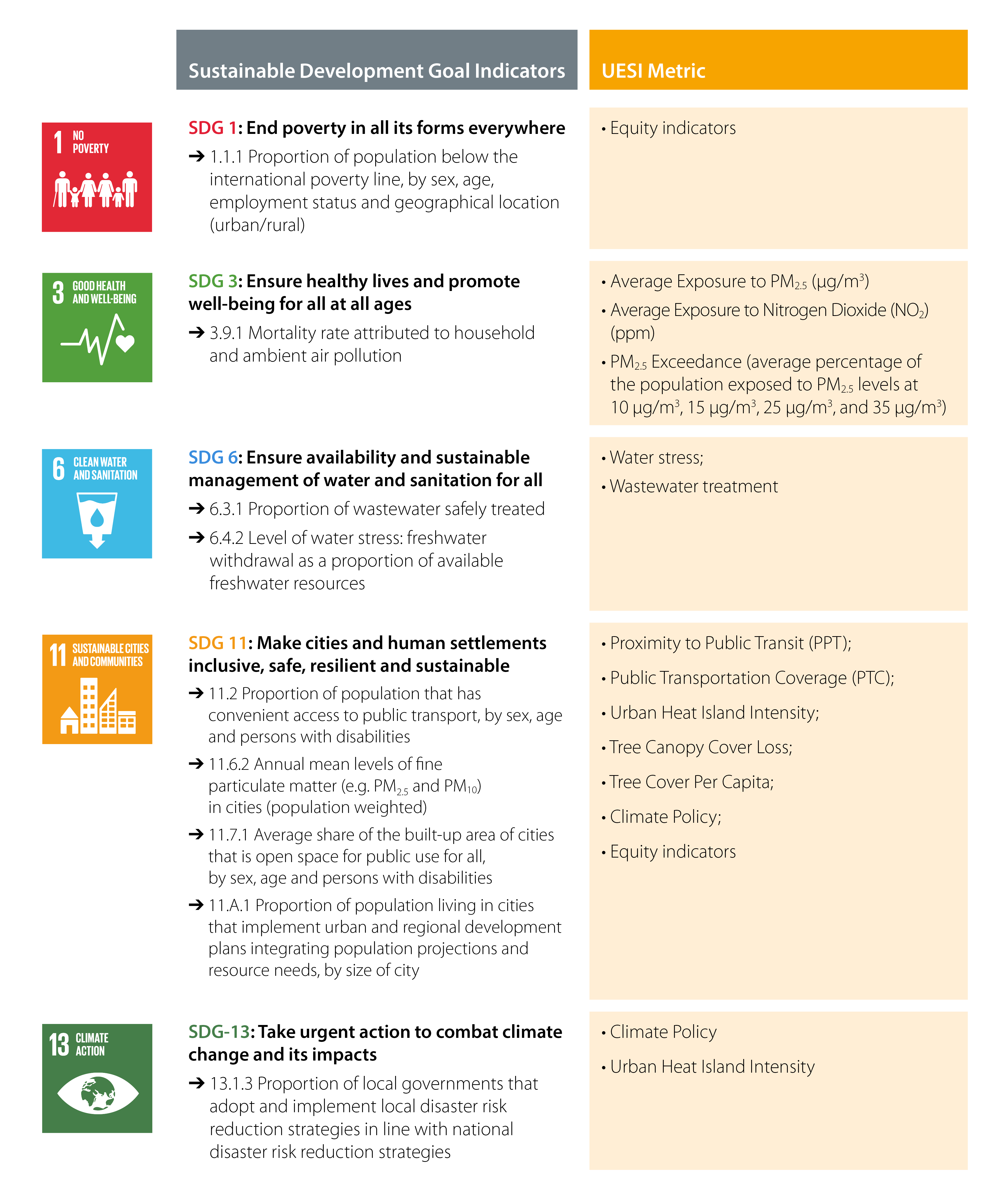 Table 1. Sustainable Development Goal indicators related to the environmental metrics included in the UESI. Source: UN Sustainable Development Knowledge Platform. 1 UN Sustainable Development Knowledge Platform. Available: https://sustainabledevelopment.un.org/.
4) Focus on outcome, not process, indicators
Targeting policymakers, we designed our framework and indicators to measure outcomes where possible, allowing local managers to address areas of needed improvement in locally-sensitive ways. With the exception of the Climate Policy indicator, UESI indicators do not measure policy responses such as public expenditure on roads.
5) Reproducibility and transparency
We provide a clear and detailed report on the chosen datasets, methodology, framework, and indicators. Access to data in easily accessible formats will be important in ensuring transparency, reproducibility, and relationship building. Ensuring the data is accessible allows individuals and institutions to access the aggregated data to investigate their own research questions. All data is available on our web portal.
Constructing the UESI
The UESI framework was developed through a multi-step stakeholder engagement process that involved input from academic researchers, urban planners, practitioners, and city representatives. The starting point for the environmental issues we selected was drawn from the 2016 Environmental Performance Index (EPI), a biennial ranking that evaluated national environmental performance in 9 high-priority issue areas (e.g., Air and Water Quality, Biodiversity and Habitat Protection, Forests, Fisheries, Agriculture, Climate Change and Energy, Environmental Health). We then conducted a comprehensive literature review of existing urban environmental sustainability metrics to evaluate prior work and where we could add value. This process also involved reviewing the environmental justice and social equity literature from a multi-disciplinary angle (see Equity and Social Inclusion issue profile) in order to design indicators that incorporate an equity lens in environmental performance. In the end, the resulting UESI framework and indicators represent a trade-off between a scientific underpinning and available data, as we require neighborhood-scale data available for most of the indicators, except for the Water Indicators (Water Stress and Wastewater Treatment) and for the Climate Policy indicators, which are city-wide and not part of the equity calculations.
Filtering ‘non-urban’ neighborhoods
Due to the need to integrate both environmental and socioeconomic data for the analysis, the UESI used primarily the officially determined administrative divisions of a city as the spatial units for the calculation of the spatially explicit environmental indicator alongside its corresponding population and income information. However, we identified that in many cases the defined boundaries of a city did not necessarily correspond exclusively to an urban area, and included non-urban areas such as sparsely populated areas, rural sections or even wildlife conservation areas.
As a result of this preliminary analysis, and due to the need to maintain a certain level of homogeneity within the districts analyzed within a city, we performed a process to identify and filter urban areas from non-urban areas, since the inclusion of non-urban areas in the UESI calculation would create unintended results in the equity analysis and the performance scores, by either rewarding or penalizing some cities, depending on the indicator.
Building on the criteria used by different organizations, like the US Census Bureau or UN-Habitat, we applied a statistical clustering process based on a combination of land cover data, population density,, the relative distances of the neighborhood to the city center, the proportion of the population of the neighborhood to the total population of the city, and the proportion of the neighborhood area to the total city area to classify all neighborhoods and differentiate entirely or partially urbanized areas, rural zones, as well as certain areas that include large non-impervious areas that are functionally part of the city, such as large parks near the boundaries of a city’s urban core. By the end of the process we identified and filtered around 1,000 neighborhoods that were entirely rural or mostly rural when compared to the rest of our UESI neighborhoods, representing around 6.9% of the initial set of city neighborhoods. The identified rural or mostly rural include areas such as the Western Water Catchment in Singapore, Pachacamac in Lima, El Esparragal in Murcia, Chunan County in Hangzhou, Mentougou in Beijing, and some Census Tracts in cities like Albuquerque, Las Vegas, Charlotte and others. Some of these examples can be seen in Figure 2, and further details on the approach can be explored in Box 2: Identifying Non-Urban areas for the UESI.

Figure 2. Relevant examples of non-urban neighborhoods (Blue) alongside its surrounding urban areas (Red): a) Western Water Catchment and Lim Chu Kang in Singapore; b) El Esparragal in Murcia; c) Census Tract 40.01 and 8.01 in Albuquerque; d) Mentougou in Beijing. Neighborhoods shaded Blue were removed from the final analysis since they were determined to be non-urban. Neighborhoods shaded Red were kept.
Box 2: Identifying Non-Urban areas in Cities
Like socioeconomic and environmental data, the spatial boundaries of the cities are also collected from multiple data sources such as city governments, statistical offices, or national open portals, as well from crowdsourced repositories such as Open Street Maps. Consequently, the spatial units for a neighborhood for each city can be very different. For example, the US city neighborhoods are closely related to statistical units generated from the US Census Bureau that are very small in heavily populated areas and larger in sparsely populated zones. On the other hand, in many other cities, like those in Asia, Latin America, Africa, and some European cities, the highest disaggregation available are exclusively based on the administrative boundaries established by each city, such as districts or parishes, creating very heterogeneous neighborhood units with varying levels of population, urbanization, and total area. In the light of the high level of variability of all the collected neighborhoods, it is not possible to use thresholds of some variables, like population density, to differentiate between primarily urban neighborhoods from non-urban ones.
Building on our previous experience, as well as relevant definitions and criteria for reputable organizations like the US Census Bureau, OECD, and UN-Habitat, we developed a clustering approach to differentiate rural neighborhoods from the entirely or mostly urban areas within our dataset. Our approach uses hierarchical clustering to identify a total of 28 clusters, 7 of which are associated to entirely rural or mostly rural areas within the dataset identified by low values of population density, higher distance to the center of the urban area, high area, and low proportion of impervious surface. An example of some of the most relevant clusters and their scaled variables can be seen in the figure below.

Figure 3. Relevant city typologies resulting from the clustering method applied to the UESI.
The results of our clustering approach allows us to identify groups of entirely rural or mostly rural neighborhoods, which might be a part of the administrative boundaries of the city government but are not fundamentally a part of the city in question. In the “Rural” Cluster we found many neighborhoods with very high individual areas, very low urbanized proportions, and low population count and density located in a variety of cities such as Brisbane, Rio de Janeiro, Orleans, Singapore, Atlanta, and Houston. Some more extreme case are part of the “Large Rural” cluster that includes even larger areas such as mountainous regions and natural reserves located in cities such as Hulumbeir, Chengdu, Qinhuangdao, and Dalian in China that are under the city’s government jurisdiction but not a part of the actual urban extent.
Finally, our clustering also allowed us to differentiate some zones that are not entirely urbanized or that include some non-urban zones that are functionally part of the cities and that should be considered as part of their extent even if they have a lower population density than some of the entirely urban zones because they provide some effective benefits to the city such as parks or access to recreational spaces. The “Functionally Urban” Cluster includes neighborhoods in cities like Johannesburg, Atlanta, New York, San Francisco, Sao Paulo, Oslo, and Amsterdam.
Use of Google Earth Engine for Computation
To scale up our analysis from both the original 32 pilot cities and the 162 in the second version of the UESI, we leverage the capabilities of Google Earth Engine, a cloud-computing platform for global scale geospatial analysis to process global data, and also provide a replicable method that allowed us to incorporate 121 new cities for a total of 283 cities in this version of the UESI.
UESI Environmental Performance Score and Environmental Equity Indicators Calculation
We present the UESI data in multiple formats recognizing that not all users experience and require information in the same way.The data available for the UESI includes the raw values in native units, which provide a largely unadulterated view of how neighborhoods and cities perform, as well as environmental performance scores for each category and an aggregated performance score for each city.
The environmental performance scores are transformed values using a “proximity to target” (Box 3: Measuring Environmental Performance: Proximity-to-Target) method and assess how close or far neighborhoods and cities are to achieving an identified policy target. The targets are high performance benchmarks or established scientific thresholds, such as the benchmark for exposure to fine particulate pollution is 10 μg/m3, a threshold set by the World Health Organization as safe exposure. A high-performance benchmark can also be determined through an analysis of the best-performing cities in the UESI. Some of our indicators set benchmarks, for example, at the 95th percentile of the range of data. Scores are then converted to a scale of 0 to 100 by simple arithmetic calculation, with 0 being the farthest from the target and 100 being the closest (Box 2). In this way, scores convey analogous meaning across indicators, policy issues, and throughout the UESI.
In addition, a significant contribution of the UESI is centered in its equity indicators, constructed from a Concentration Curve (See Equity Issue Profile) , that evaluate the equity in the allocation of an environmental benefit or hazard in relation to the income distribution within each city. Four categories included in the UESI have an associated Concentration Index that allows the user to evaluate if less affluent citizens might be exposed to a higher proportion of an environmental hazard, or have less access to an environmental benefit.
Finally, although many environmental scores and indices such as the EPI focus their communication and contribution in a single index based on the weighted aggregation of their scores into a composite index the UESI’s main approach is not centered in combining all of metrics into a single composite score.We keep the UESI scores disaggregated by issue based on the range of environmental performance observed at the neighborhood scale and because the cities in the UESI include cities at different levels of development. Our aim is to illustrate the range of urban sustainability solutions and challenges, not to “name and shame” or rank cities.
That being said, some figures, particularly those in the Key Findings section, include aggregated environmental performance and inequality indexes (for example, Figures 3 and 5), which represent a weighted average of how a city performs on the underlying indicators. All issue categories (e.g., Air Quality, Climate Change, and Urban Ecosystem) are weighted equally (1), with one exception – the Public Transportation Category – which has a lower weight than the other three categories (0.5) due to the limitations and potential issues related to data quality of the source dataset of this category when compared to the rest given that unlike other categories that are sourced from peer-reviewed datasets, the Public Transportation source is fundamentally crowdsourced (OSM) (See Transportation – Box 2). Within each issue category, individual indicators are weighted equally. Figure 4 presents a graphical summary on the weighting schemes for both the aggregated performance and concentration indices.
The city-wide indicators (Water Stress, Wastewater Treatment, and Climate Policy) are not included as part of our evaluation of each city’s equity indicators or aggregated environmental performance or inequality indices, since they are not available for all cities at this time and don’t provide disaggregated information to assess their within-city variability.

Figure 4: Weighting schemes used for calculation of the Aggregated Performance Index (a) and the Aggregated Concentration Index (b). All issue categories (Air Quality, Climate Change, and Urban Ecosystem) are weighted equally (1), with one exception, Public Transportation which is weighted as 1/2. Within each issue category, the indicators are weighted equally.
Box 3: Measuring Environmental Performance: Proximity-to-Target
There are many ways to summarize and transform raw data to make it comparable. Targets are set by policy goals (e.g., in the case of the Tree Cover per capita target that uses a UN SDG goal of 15 meters per capita), established scientific thresholds (e.g., in the case of the PM2.5 indicator that uses the World Health Organization’s 10 microgram/m3 limit for exposure), or an analysis of the top performers (e.g., the top 5th percentile of the distribution of scores). Each indicator is transformed given a score from a scale of 0 (worst performer or those at the low performance benchmark) to 100 (best performer or those at the top performance benchmark).
")
Figure 5. Illustration of the proximity to target methodology (Source: adapted from Hsu et al., 2013).2Hsu, A., Johnson, L. A., & Lloyd, A. (2013). Measuring progress: a practical guide from the developers of the environmental performance index (EPI). New Haven: Yale Center for Environmental Law & Policy.
References:
Center for International Earth Science Information Network – CIESIN – Columbia University. 2018. Gridded Population of the World, Version 4 (GPWv4): Population Count, Revision 11. Palisades, New York: NASA Socioeconomic Data and Applications Center (SEDAC). https://doi.org/10.7927/H4JW8BX5
Cooper, M.J., Martin, R.V., Hammer, M.S. et al. Global fine-scale changes in ambient NO2 during COVID-19 lockdowns. Nature 601, 380–387 (2022)
Kummu, M., Taka, M., & Guillaume, J. H. (2018). Gridded global datasets for gross domestic product and Human Development Index over 1990–2015. Scientific data, 5, 180004.
Gémes, O., Tobak, Z., & Van Leeuwen, B. (2016). Satellite based analysis of surface urban heat island intensity. Journal of environmental geography, 9(1-2), 23-30.
Stone, B., Hess, J. J., & Frumkin, H. (2010). Urban form and extreme heat events: are sprawling cities more vulnerable to climate change than compact cities?. Environmental health perspectives, 118(10), 1425.
Hsu, A., D. Esty, M. Levy, A. de Sherbinin, et al. 2016. The 2016 Environmental Performance Index Report. New Haven, CT: Yale Center for Environmental Law and Policy. https://doi.org/10.13140/RG.2.2.19868.90249.
Thomas, R., Hsu, A., & Weinfurter, A. (2020). Sustainable and inclusive – Evaluating urban sustainability indicators’ suitability for measuring progress towards SDG-11. Environment and Planning B: Urban Analytics and City Science, 239980832097540. doi:10.1177/2399808320975404.
https://www2.census.gov/geo/pdfs/reference/ua/Census_UA_CritDiff_2010_2020.pdf
https://unhabitat.org/sites/default/files/2020/06/city_definition_what_is_a_city.pdf
Gorelick, Noel, et al. “Google Earth Engine: Planetary-scale geospatial analysis for everyone.” Remote sensing of Environment 202 (2017): 18-27.
World Health Organization. (2006). WHO Air quality guidelines for particulate matter, ozone, nitrogen dioxide and sulfur dioxide-Global update 2005-Summary of risk assessment, 2006. Geneva: WHO.
Hsu, A., Johnson, L. A., & Lloyd, A. (2013). Measuring progress: a practical guide from the developers of the environmental performance index (EPI). New Haven: Yale Center for Environmental Law & Policy.