Issue Profile
Climate Change & Urban Heat Island effect
Cities are contributing to global warming as well as developing policies to lessen their climate impact. The Climate Change category tracks cities’ Urban Heat Island intensity and their mitigation and adaptation strategies.
Chapter Authors
TC Chakraborty
Yihao Xie
Saskia Comess
The Climate Change category includes two indicators: Urban Heat Island (UHI) intensity and Urban Climate Policy Score. UHI intensity measures the annual mean difference in daytime and nighttime surface temperatures between urban land cover and non-urban land cover within the city, in degrees Celsius (°C) for 2016.
For the UESI pilot cities, the Climate Policy Score assesses cities’ efforts to reduce their contribution to climate change as well as to adapt to a changing climate.
Urban Heat Island intensity has both public health and economic consequences. As the world warms, heat waves are expected to become more frequent, and UHI amplifies this effect in urban areas, exacerbating heat stress and accounting 1Schär, C., Vidale, P. L., Lüthi, D., Frei, C., Häberli, C., Liniger, M. A., & Appenzeller, C. (2004). The role of increasing temperature variability in European summer heatwaves. Nature, 427(6972), 332-336.for a large proportion of deaths during heat waves. 2Heaviside, C., Vardoulakis, S., & Cai, X. M. (2016). Attribution of mortality to the Urban Heat Island during heatwaves in the West Midlands, UK. Environmental Health, 15(1), S27.Hot and arid communities are frequently water-stressed, and higher temperatures in these regions can aggravate water scarcity by spurring residents’ increased water consumption. 3Guhathakurta, S., & Gober, P. (2007). The impact of the Phoenix urban heat island on residential water use. Journal of the American Planning Association, 73(3), 317-329.By enhancing chemical reaction rates, urban heat can also increase production of secondary pollutants,4A primary pollutant is an air pollutant emitted directly from a source, such as a car’s tailpipe. A secondary pollutant forms when other pollutants (primary pollutants) react chemically in the atmosphere. Source: European Union. Glossary. Available at: https://ec.europa.eu/health/scientific_committees/opinions_layman/en/indoor-air-pollution/glossary/pqrs/primary-pollutant-secondary-pollutant.htm (accessed 5 August 2018). such as ground-level ozone, worsening local air quality. 5Sarrat, C., Lemonsu, A., Masson, V., & Guedalia, D. (2006). Impact of urban heat island on regional atmospheric pollution. Atmospheric environment, 40(10), 1743-1758.Since ground-level ozone is a precursor to photochemical smog, UHI can have a particularly detrimental impact in cities already struggling with this issue. However, warmer surfaces can also increase convective mixing, which can reduce the concentration of primary pollutants; put another way, UHI can help prevent temperature inversions, which trap warm air – and pollutants – beneath a layer of cold air.6Li, H., Meier, F., Lee, X., Chakraborty, T., Liu, J., Schaap, M., & Sodoudi, S. (2018). Interaction between urban heat island and urban pollution island during summer in Berlin. Science of the Total Environment, 636, 818-828.
The UHI effect also has a wide range of economic impacts. Urban heat increases cooling and reduces heating requirements, which, in turn, may increase or decrease electricity use. 7Santamouris, M. (2014). Cooling the cities–a review of reflective and green roof mitigation technologies to fight heat island and improve comfort in urban environments. Solar Energy, 103, 682-703.A large number of studies have investigated the possible effects of UHI on power demand. 8Santamouris, M., Cartalis, C., Synnefa, A., & Kolokotsa, D. (2015). On the impact of urban heat island and global warming on the power demand and electricity consumption of buildings—A review. Energy and Buildings, 98, 119-124.In London, urban heat increases cooling load by 25 percent and reduces heating load by 22 percent on an annual basis. 9Kolokotroni, M., Zhang, Y., & Watkins, R. (2007). The London Heat Island and building cooling design. Solar Energy, 81(1), 102-110.In Greek cities, UHI doubled the cooling load, while lowering the heating load by 30 percent. 10Santamouris, M., Papanikolaou, N., Livada, I., Koronakis, I., Georgakis, C., Argiriou, A., & Assimakopoulos, D. N. (2001). On the impact of urban climate on the energy consumption of buildings. Solar energy, 70(3), 201-216.A literature review of similar studies shows the UHI effect increases cities’ average energy load by 11 percent, accounting for both the decreased heating and increased cooling loads.11Santamouris, M. (2014). On the energy impact of urban heat island and global warming on buildings. Energy and Buildings, 82, 100-113. Higher urban temperatures can also reduce the efficiency and life span of devices, such as cooling systems, automobile engines, and electronic appliances, creating costs of hundreds of million dollars for some cities. 12Miner, M. J., Taylor, R. A., Jones, C., & Phelan, P. E. (2017). Efficiency, economics, and the urban heat island. Environment and Urbanization, 29(1), 183-194.Additionally, UHI can exacerbate the contributions of heat stress to work absenteeism and productivity loss.13Zander, K. K., Botzen, W. J., Oppermann, E., Kjellstrom, T., & Garnett, S. T. (2015). Heat stress causes substantial labour productivity loss in Australia. Nature Climate Change, 5(7), 647-651.14Estrada, F., Botzen, W. W., & Tol, R. S. (2017). A global economic assessment of city policies to reduce climate change impacts. Nature Climate Change, 7(6), 403-40 In short, UHI can dramatically shape the lives of its urban residents, but these impacts are heavily dependent on the city in question and can vary substantially across urban areas.
For the UHI intensity indicator, measurements of Land Surface Temperature (LST) are derived from the Moderate Resolution Imaging Spectroradiometer (MODIS) sensor on board the Aqua satellite 15Wan, Z. (1999). MODIS land-surface temperature algorithm theoretical basis document (LST ATBD). Institute for Computational Earth System Science, Santa Barbara, 75.16Strahler, A. S., Moody, A., Lambin, E., Huete, A., Justice, C. D., Muller, J. P., … & Wan, Z. (1994). MODIS land cover product: Algorithm theoretical basis document. and measurements of land cover are derived from the European Space Agency’s Climate Change Initiative land cover product.17Bontemps S, Defourny P, Radoux J, Van Bogaert E, Lamarche C, Achard F and Zülkhe M 2013 Consistent global land cover maps for climate modelling communities: current achievements of the ESA’s land cover CCI Proc. ESA Living Planet Symp. pp 9–13 The MODIS satellite gathers daytime values at 1:30 pm local time, and nighttime values at 1:30 am local time. For the UESI, we only consider the cloud-free MODIS pixels with an uncertainty of less than 3 °C for 2016. For each city, the reference LST is defined as the mean of the non-urban, non-water pixels. This reference value is subtracted from the mean LST of all the urban pixels in each neighborhood to get the UHI of the neighborhoods of a city. The method used in the UESI is a modified version of the simplified urban-extent (SUE) algorithm adjusted for neighborhood-level UHI detection.18Chakraborty, T. & Lee, X. (2018). A Simplified Urban-Extent Algorithm to Characterize Surface Urban Heat Islands on a Global Scale and Examine Vegetation Control on their Spatiotemporal Variability, International Journal of Applied Earth Observation and Geoinformation.
There are currently no standardized targets for the UHI effect since its consequences vary on a city-by-city basis. For instance, public health consequences, like increased heat stress, depend on the background climate of the city and the physiological adaptation of the people living in that area. But, for most locations, the goal is to reduce and, if possible, completely negate the UHI. In addition, the change in the UHI intensity over time and the variation of the UHI intensity within neighborhoods is important to quantify, since they represent how the urban heat stress has worsened or improved over time, and how it disproportionately affects populations within the same city.

Figure 1a. The urban heat island effect in practice. As areas become more built up, excess heat is trapped in developed areas, increasing their temperature compared to rural areas in the same climate.
Description
Urban Heat Island
The UHI effect is one of the oldest known consequences of urbanization. The phenomenon was observed for the first time over a century ago, and is currently one of the major research themes in urban climatology. 19Howard, L. (1833). The climate of London, vols. I–III. London: Harvey and Dorton.The act of urbanization replaces natural surfaces with built-up structures. This conversion changes the radiative, thermal, and aerodynamic properties of the surface, which modifies the energy balance over urban surfaces. 20Oke, T. R. (1982). The energetic basis of the urban heat island. Quarterly Journal of the Royal Meteorological Society, 108(455), 1-24.Urbanization involves the replacement of vegetated land surface with a built-up structures, which are predominantly composed of asphalt (for highways) and concrete (for buildings). Concrete is slightly lighter in color (has a higher albedo) than vegetation, while asphalt is darker and has a lower albedo than vegetation. Thus, concrete reflects a higher percentage of solar radiation than vegetation, while asphalt absorbs more radiation than natural surfaces. Depending on the percentage of concrete and asphalt in an urban area, it might absorb less or more radiation than it would in its natural state. Urbanization also leads to the replacement of vegetation with built-up structures. This shift reduces the evaporative cooling vegetation provides, further increasing heat build-up in urban areas. There are other city-specific factors that modulate UHI intensity, including: the higher thermal mass of built-up structures; the ability of urban canyons and urban haze to trap outgoing longwave radiation; and the difference in surface roughness between the city and its surroundings, illustrated in Figure 121Oke, T. R. (1981). Canyon geometry and the nocturnal urban heat island: comparison of scale model and field observations. International Journal of Climatology, 1(3), 237-2522Cao, C., Lee, X., Liu, S., Schultz, N., Xiao, W., Zhang, M., & Zhao, L. (2016). Urban heat islands in China enhanced by haze pollution. Nature communications, 7.23Zhao, L., Lee, X., Smith, R. B., & Oleson, K. (2014). Strong contributions of local background climate to urban heat islands. Nature, 511(7508), 216-219..

Figure 1b. Factors causing UHI. Adapted from (Kleerekoper et al., 2012)24Kleerekoper, L., Van Esch, M., & Salcedo, T. B. (2012). How to make a city climate-proof, addressing the urban heat island effect. Resources, Conservation and Recycling, 64, 30-38..
There are two primary approaches to measuring UHI intensity. The canopy UHI measures the difference in air temperature between the urban region and its surrounding “background” or non-urban region. The surface UHI measures the difference in the surface temperature between the urban and “background” regions, often using satellite data. Our UHI indicator focuses on the surface UHI – the difference in daytime and nighttime mean surface temperatures – since air temperature measurements are usually not available for cities (see Box 1, The Rural Reference: Defining the Urban Heat Island Magnitude).
Box 1. The rural reference: Defining the magnitude of urban heat island
All Urban Heat Island (UHI) estimates use the difference in temperature (surface or air) between the urban area and a rural reference area. For canopy UHI, which measures air temperature 1.5 to 2 meters above the ground, this reference is a rural station where air temperature is measured. For surface UHI, which measures surface temperatures, the reference is provided by the surface temperature of the area outside the urban boundary. 25Martin-Vide, J., Sarricolea, P., & Moreno-García, M. C. (2015). On the definition of urban heat island intensity: the “rural” reference. Frontiers in Earth Science, 3, 24.Since canopy UHI studies are done on an individual basis, there are frequently inconsistencies in the choice of the rural stations, both within and between cities. A recent critique of the UHI literature found that roughly half of canopy UHI studies were not robust, with issues ranging from ignoring local weather effects to a lack of site and instrument metadata. 26Stewart, I. D. (2011). A systematic review and scientific critique of methodology in modern urban heat island literature. International Journal of Climatology, 31(2), 200-217.
Researchers usually define a buffer zone around urban areas to represent the rural reference for surface UHI determination. The use of the buffer zone can create problems in getting a consistent measure of the surface UHI magnitude across cities. A recent study found that the footprint or extent of the surface UHI can be two to three times the area of the city, which is much larger than the area typically defined as the buffer zone. 27Zhou, D., Zhao, S., Zhang, L., Sun, G., & Liu, Y. (2015). The footprint of urban heat island effect in China. Scientific reports, 5, p.11160.Mechanistically, this is mainly because warm air often travels from urban to rural areas. It could also be because the datasets used to define the urban area may be old and do not capture more recent urban sprawl. Moreover, if one city is downwind of another, advection can change the temperature of the rural reference, and thus, the UHI magnitude. 28Heaviside, C., Cai, X. M., & Vardoulakis, S. (2015). The effects of horizontal advection on the urban heat island in Birmingham and the West Midlands, United Kingdom during a heatwave. Quarterly Journal of the Royal Meteorological Society, 141(689), 1429-1441.A recent study on the UHI of a subtropical Indian city found that irrigation patterns around the rural reference can affect the seasonal value of the rural surface (or air) temperature, and thus, the measured surface and canopy UHI. 29Heaviside, C., Cai, X. M., & Vardoulakis, S. Finally, the area of the buffer zone around cities of different sizes should be different, since a city’s UHI footprint is a function of the city area. For instance, larger cities should have higher buffer zones since the localized thermal anomaly – the UHI – extends further from the city boundary. However, the impact of city size is not normally considered in most existing UHI studies.
For all these reasons, instead of using buffer zones, we determine the surface UHI in the UESI using a simplified urban-extent (SUE) algorithm, modified to be implemented at the neighborhood scale. Comparing our results with the UHI values calculated using 3 km buffers confirms that this algorithm can capture the spatial variation of the UHI (see Figure 1). The references produced by the two approaches differ by a constant value specific to each city. The original SUE algorithm uses the difference in mean land surface temperature over the MODIS-derived urban pixels and the MODIS-derived non-urban pixels within the urban boundary to define the UHI.30Chakraborty, T. & Lee, X. (2018). A Simplified Urban-Extent Algorithm to Characterize Surface Urban Heat Islands on a Global Scale and Examine Vegetation Control on their Spatiotemporal Variability, International Journal of Applied Earth Observation and Geoinformation In this version, the European Space Agency’s Climate Change Initiative land cover data are used instead of the MODIS land cover product. At the neighborhood scale, since some urban neighborhoods may not have non-urban pixels, the mean surface temperature over the non-urban pixels for the whole city is subtracted from that over the urban pixels in each neighborhood to determine the surface UHI magnitude for that neighborhood. In other words, the SUE finds the difference in temperature between the built-up and non-built-up surfaces within each urban boundary. The SUE algorithm may underestimate the surface UHI magnitude compared to methods that use a buffer zone, but it reduces the uncertainty that can arise from seasonal changes in rural land use31Chakraborty, T., Sarangi, C., & Tripathi, S. N. (2017). Understanding Diurnality and Inter-Seasonality of a Sub-tropical Urban Heat Island. Boundary-Layer Meteorology, 163(2), 287-309. and different urban footprint sizes.
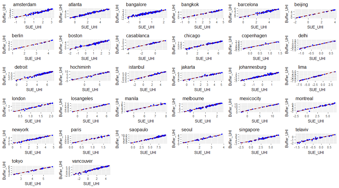
Figure 2. Relationship between neighborhood-level UHI calculated in this study and that calculated using a 3 km buffer around the UESI pilot cities.
Ideally, the SUE algorithm should be used for urban clusters created from land use datasets based on spectral classification – that is, datasets that take into account the radiative properties of the land surface. The UESI currently uses politically-defined city boundaries, which are created by local municipalities and might encompass a whole district in the case of one city, while only including the urban core for another. Since these boundaries differ so widely, the surface UHI magnitude determined here should not be compared between cities. However, the surface UHI value can give a good indication of the variation in surface temperature between neighborhoods for a single city.
Urban Heat Island and Urban Policy
The UHI effect, and by extension, its consequences, all stem from urban-scale changes. Thus, these effects can be prevented through more-informed policymaking and city planning. There are various ways to geoengineer urban areas to lessen the magnitude of the UHI. For instance, urban temperatures can be reduced by increasing the reflectivity of the city or by increasing evaporative cooling over urban surfaces. Four main methods are normally used to mitigate the UHI:
- White roofs: White roofs can increase the surface albedo, reflecting more of the sun’s radiation back to space.
- Green spaces: Green spaces can increase evaporative cooling over land, thus reducing the average temperature over cities.
- Green roofs: Green roofs are similar to green spaces, but can directly reduce the temperature over built-up structures.
- Reflective pavements: Like white roofs, reflective pavements also increase the surface albedo, and thus, reduce the absorption of radiation by urban areas.
Previous studies have quantified the impact of these methods on the UHI magnitude for individual cities.32Rizwan, A. M., Dennis, L. Y., & Chunho, L. I. U. (2008). A review on the generation, determination and mitigation of Urban Heat Island. Journal of Environmental Sciences, 20(1), 120-128.A recent large-scale study on UHI mitigation strategies over 57 cities in Canada and the U.S. showed that the combination of white roofs, reflective pavements, and green roofs can negate the effect of both global warming and the UHI for many cities.33Zhao, L., Lee, X., & Schultz, N. M. (2017). A wedge strategy for mitigation of urban warming in future climate scenarios. Atmospheric Chemistry and Physics, 17(14), 9067-9080. These mitigation strategies involve changing the surface cover, and can be implemented for existing cities. Rapidly expanding cities can also opt for large-scale engineering of the urban structure to reduce the UHI intensity. For instance, zoning policies can increase the horizontal dissipation of heat by staggering building heights against the prevailing winds.34oritizing urban sustainability solutions: coordinated approaches must incorporate scale-dependent built environment induced effects. Environmental Research Letters, 10(6), 061001.
While solving climate change requires global effort and cooperation between different countries, it is possible to temporarily shield urban residents from some of the consequences of climate change by enacting policies designed to curb the UHI. With around 66 percent of the global population expected to live in urban areas by 2050, mitigating urban heat can provide large benefits for both human health and the economic growth of cities. In this regard, city-level policies, enacted in tandem with multi-scale adaptation strategies, will become important to ensuring the sustainable growth of urban areas in a rapidly warming world.
UHI and Equity Results for Pilot Cities
The UESI pilot cities show a large range of daytime UHI values, from approximately 0 °C to above 7 °C (see Figure 2). Most of the cities show higher UHI values in the city core. Some of the neighborhoods, including several Johannesburg neighborhoods and some of Beijing and Vancouver’s outer neighborhoods, have negative daytime UHI, meaning parts of the city are cooler than their reference non-urban areas. For instance, some of Beijing’s neighborhoods, especially those near the edges of the city, tend to have more green space, and more rural or suburban land use, than the city as a whole, so are cooler than the average city neighborhood. Among the pilot UESI cities, Sao Paulo shows the highest mean daytime UHI, followed closely by Mexico City and Manila. Johannesburg shows no significant UHI during the day.

Figure 3: Daytime UHI intensity of pilot cities as calculated in the UESI using the modified SUE algorithm. The number in the circle is the mean daytime UHI for the city, while the error bars represent the standard deviation of UHI values across different neighborhoods of the city.

Figure 4. UHI typology quadrant plot. The plot considers the Income Gini and UHI Concentration Index to define four quadrants. The Income Gini Values represent the distribution of wealth across the population and range in value from 0 to 1. A Gini value of 0 indicates a perfectly equal distribution of income across the population, while a high Gini value (out of a maximum of 1) suggests a highly unequal distribution of wealth. The Environmental Concentration Index (ECI) measures the variation in UHI in response to income. Negative ECI values indicate that the environmental burden is allocated on the poorest citizens, while a positive ECI indicates that the environmental burden is allocated on the wealthier citizens. The size of the dots represents the extent of UHI intensity (in C). (See the Equity and Social Inclusion Profile for a more detailed description of this plot).
Figures 4 and 5 capture the income inequality within the UESI pilot cities using the income GINI coefficient, as well as the degree to which neighborhoods’ UHI intensity is sensitive to income, using a concentration index. Cities like Los Angeles, Vancouver, Detroit, and Atlanta fall into the second quadrant in the UESI’s typology comparing relationships between income and environmental outcomes across cities. These cities have low income inequality, but a greater UHI burden falls on the poorer sections of society. For cities like Bangkok, Sao Paulo, Beijing, and Singapore, the rich are affected more by the UHI, possibly because the city core, with high UHI values, is populated by the wealthy section of society. In Johannesburg, there is high income inequality, which is further compounded by a disproportionate heat island burden for the lower-income group.35Chakraborty, T., Hsu, A., Manya, D., & Sheriff, G. (2019). Disproportionately higher exposure to urban heat in lower-income neighborhoods: a multi-city perspective. Environmental Research Letters, 14(10), 105003. For a detailed look at the ways some cities address the intersection of urban heat and equity, see Box 2 on The Urban Heat Island Effect in Montreal.

Figure 5. Environmental and Income Distribution Curves for selected cities. These plots show the concentration distributions of UHI intensity (e.g., the concentration curve) and income (e.g., the Lorenz curve) throughout neighborhoods in cities. Deviations from the dotted line (e.g., the line of perfect equity) illustrate cities that are less equitable in their distribution of UHI intensity. Concentration curves above the line of equity indicate the environmental burden is more heavily allocated to those with less income; concentration curves below the line of equity indicate that the environmental burden is more heavily allocated to those with greater income. (See the Equity Indicator Profile for a more detailed description of this plot, and the UESI Cities Page to explore the income and distribution curves for all UESI cities).
Box 2. The Urban Heat Island Effect in Montréal
The summer of 2019 was the hottest one on record for the Northern Hemisphere, where 90% of the Earth’s population lives.36Rice, Doyle. “It Was the Hottest Summer on Record for the Northern Hemisphere.” USA Today, Gannett Satellite Information Network, 16 Sept. 2019, https://www.usatoday.com/story/news/nation/2019/09/16/global-warming-earth-had-second-hottest-summer-record/2342104001/. In France alone, the mortalities of 1,435 people were linked to a pair of heat waves that occurred in June and July 2019.37United Nations, Department of Economic and Social Affairs, Population Division (2018). The World’s Cities in 2018—Data Booklet (ST/ESA/ SER.A/417). As our planet warms, we must be prepared to deal with the fallout of rising temperatures. More than half of the world’s population lives in urban areas, which will place an enormous amount of pressure on how we should design and run our cities in order to deal with urban heat.38Berlinger, Joshua. 2019. “Nearly 1,500 Deaths Linked to French Heat Waves.” CNN. Cable News Network. September 9, 2019. https://www.cnn.com/2019/09/08/europe/france-heat-wave-deaths-intl-hnk-scli/index.html. In cities, the urban heat island effect puts some residents at greater risk to the detrimental effects of extreme heat. The urban heat island effect is a phenomenon where some urban areas are significantly higher in temperature than surrounding rural areas.39.S. Environmental Protection Agency. 2008. Reducing urban heat islands: Compendium of strategies. Draft. https://www.epa.gov/heat-islands/heat-island-compendium.
In order to understand the causes and effects of urban heat, and to generate practical and impactful solutions to its hazardous outcomes, Claire Suh, a Samuel Centre for Social Connectedness Research Fellow, examined the ways urban heat island impacts the city of Montreal. Evidence was drawn from academic papers, current policies, interviews with stakeholders, census data analysis, and roundtable discussions, and then compiled into an accessible web page: Urban Heat in Montreal.
A Range of City Climate Policies
Municipal actors play an increasingly important role in climate change mitigation. Nation-states have, until recently, been the focal points of global climate action, reporting, and target-setting. This paradigm has shifted, however, and multinational frameworks, like the UN Framework Convention on Climate Change (UNFCCC), have begun to recognize a sea change: countries are no longer the sole actors in global climate governance. Cities, regions, and states, along with businesses, investors, and civil society organizations play an increasingly prominent role in climate mitigation, adaptation and finance. The UNFCCC’s 21st Conference of Parties (COP21) negotiations, held in Paris in December 2015, codified this shift in the Paris Agreement’s text.40United Nations Framework Convention on Climate Change (UNFCCC). (2015). Adoption of the Paris Climate Agreement. And more than 400 mayors, civic leaders, and CEOs participated in the concurrent Climate Summit for Local Leaders in Paris’s City Hall.41Climate Summit for Local Leaders. United Cities and Local Governments. (2015, December 4). Retrieved January 15, 2018, from: https://www.uclg.org/en/media/events/climate-summit-local-leaders.
A special chapter on non-state (e.g., business) and subnational (e.g., cities and states) of the 2018 UN Emissions Gap Report projects that by 2030, these new climate actors could narrow the emissions gap by 0.2-0.7 gigatons (Gt) CO2 equivalent per year compared to full Nationally Determined Contribution implementation, or 1.5-2.2 Gt CO2 equivalent per year compared to current policy scenarios. 42Hsu, A., Widerberg, O., Weinfurter, A., Chan, S., Roelfsema, M., Lütkehermöller, K. and Bakhtiari, F. (2018). Bridging the emissions gap – The role of nonstate and subnational actors. In The Emissions Gap Report 2018. A UN Environment Synthesis Report. United Nations Environment Programme. Nairobi.In countries like the United States, where political events have weakened national level climate action, actors at the state, city, and businesses levels have taken up the responsibility to stay on track to meeting Paris Agreement goals. 43Data-Driven Yale. (19 September 2017). Mapping American Climate Action: Who’s Taking Charge of the Paris Agreement. Retrieved from: https://datadrivenlab.org/climate/mapping-american-climate-action-whos-taking-charge-of-the-paris-agreement/.Cities are also at the frontline of climate adaptation policies and actions, and can develop, pilot and implement targeted action plans to meet context-specific mitigation challenges.
Networks like the C40 Cities Climate Leadership Group, which includes over 90 global cities from New York to Johannesburg, and the Global Covenant of Mayors for Climate and Energy, which includes more than 8,000 cities, are connecting cities to share best practices for addressing climate change at the urban scale. In recent years, these groups have attracted more participants from a wider geographic range, while new networks and alliances continue to spring up, promoting the exchange and sharing of goals and best practices among cities. Many networks and initiatives publish their members’ emission data and detailed climate plans. A large portion of city climate action data used in this project are downloaded from climate action registries and networks like the Global Covenant of Mayors for Climate and Energy and ICLEI’s carbonn Climate Registry.
Box 3. Scoring Climate Policy in the Pilot Cities
The launch of the pilot UESI included a Climate Policy Indicator, which assessed cities’ efforts to reduce their contribution to climate change as well as to adapt to a changing climate. This indicator drew from publicly-available climate action plans that had not ended or expired in 2017, drawn from extensive searches on the UESI cities’ official websites in English and native languages, as well as from the databases of global subnational climate actor networks, such as carbonn Carbon Registry, Global Covenant of Mayors and Under2Coalition. Each pilot city’s mitigation and adaptation policies were scored according to the criteria summarized by Table 1.
|
Emission reduction |
Sectoral mitigation |
Adaptation |
Transparency and finance |
|
Timeline Pre-2020/short- (3 points), 2020-2030/medium- (2 points) and post 2030/long-term (1 point) |
Presence (1 point) and articulation (2 points) of goals in each of the following sectors: Building and Construction; Industrial; |
Presence (1 point) and articulation (2 points) of adaptation goals under each of the following themes: Infrastructure; |
Emissions inventory and data transparency (1 point for presence; 2 points for open access) |
|
Ambitious goal (1 point) |
Measuring and Evaluating mitigation actions (1 point; 2 points for evidence of actual M&E) |
||
|
Boundary (only government operations vs. city-wide) (2 points) |
Implementation status of mitigation goals (1 point) |
Implementation status of adaptation goals (1 point) |
Measuring and Evaluating adaptation actions (1 point; 2 points for evidence of actual M&E) |
|
Financing climate actions (1 point) |
Table 1. Scoring Rubric for Climate Actions for UESI Pilot Cities. Cities’ climate policies and actions were scored based on this rubric. Each category is scored only once. For example, if a city has five different climate actions in the Electricity or Energy sector, we only recorded one action, choosing the one with the highest value in our scoring system.
To collect climate action policies of the UESI cities, we conducted extensive searches on the UESI cities’ official government and environment websites in English and languages commonly-spoken in the city, and drew from global climate action databases, such as ICLEI’s carbonn Carbon Registry, the Global Covenant of Mayors for Climate and Energy, and the Under2 Coalition. While every effort was made to ensure that all climate actions and policies were recorded, we could not guarantee that the policies collected are exhaustive. The level of transparency and ease of data access differ across cities, and we incorporated this aspect into the scoring methodology. Additionally, collecting this data is extremely time and resource intensive, which is one reason it has not been replicated for all UESI cities.
Box 4. Climate Policy Performance in Pilot Cities
Table 2 summarizes the Climate Policy scores of UESI pilot cities. Overall, Melbourne, Detroit, Atlanta, Los Angeles and Boston are the top scorers, while Manila scores lowest. Bangalore, Casablanca, Delhi, and Tel Aviv are not included in the table because no publicly available climate action plan could be found. These cities receive a score of 0, although there are some indications that climate plans are in development for Tel Aviv, which joined C-40 Cities for Climate Leadership in December 201744C40 Cities for Climate Leadership. (2017). Tel Aviv Affirms Global Leadership in Taking Climate Action by Joining C40 Cities. Retrieved from: https://www.c40.org/press_releases/tel-aviv-yafo-joins-c40-cities-climate-leadership-group and is in the process of working with the group to develop its city-level climate action plan.
Amsterdam, Atlanta, Berlin, Copenhagen, Detroit, Los Angeles, London, Mexico City and New York have mitigation targets that cover a comprehensive range of time frames: pre-2020, 2020-2030 and post-2030 timeframes. Amsterdam, Beijing, Berlin, Melbourne, Jakarta, Johannesburg, Seoul and Vancouver have emission reduction targets that exceed their countries’ climate action plans, or Intended Nationally Determined Contributions (INDCs).
Most pilot UESI cities have included detailed mitigation plans and targets to improve energy efficiency and reduce emissions across different sectors. The presence and level of details of adaptation policies, however, show greater variance and are not as well documented as mitigation efforts. Notably, Seoul, Melbourne, Mexico City and Jakarta have introduced adaptation policies and detailed climate adaptation projects in their urban climate policies, therefore receiving higher scores in this category.
Vancouver has the most comprehensive monitoring and evaluation (M&E) information about its climate policies, and scored the highest under the “M&E and Finance” category. Vancouver documents its annual progress towards its climate targets, through a yearly report, and through a user-friendly online interface that tracks and quantifies the city’s progress, as shown in Figure 4. Other M&E practices adopted by UESI cities include progress reports and annual updates and iterations of existing policies.
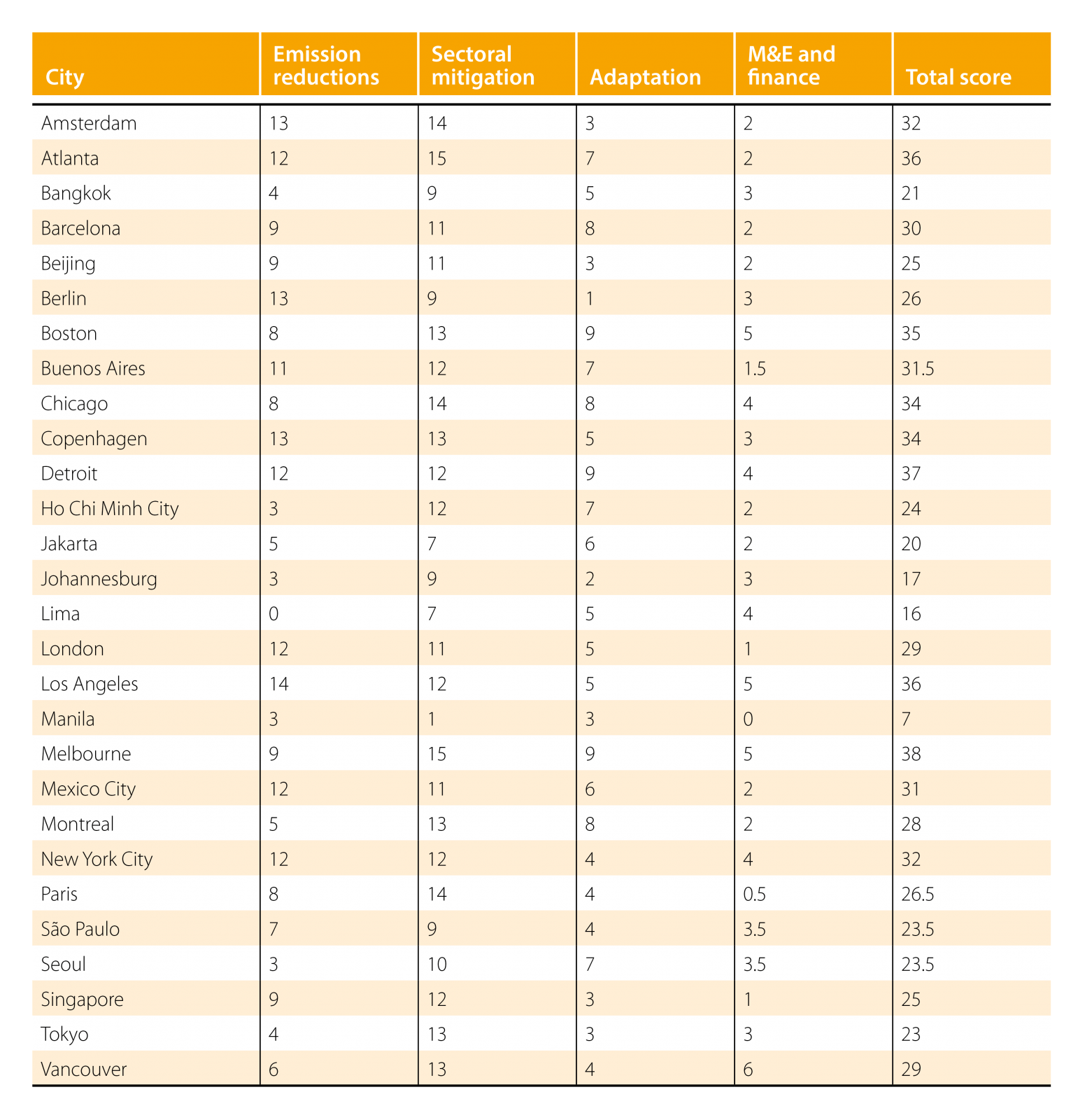
Table 2. Climate Policy Score Breakdown for the UESI pilot cities.
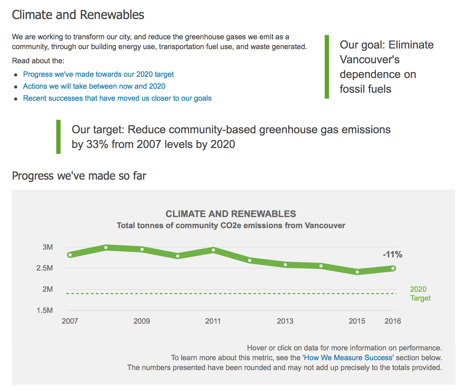
Figure 6. Screenshot of Vancouver’s Greenest City Action Plan portal, which shows progress the city has made on its climate targets. Source: http://vancouver.ca/green-vancouver/climate-and-renewables.aspx45US states, cities and businesses keep US climate action on track. (2017, September 18). Retrieved January 8 2018 from: https://www.theclimategroup.org/news/us-states-cities-and-businesses-keep-us-climate-action-track.
Box 4. Challenges of scoring cities’ climate policies on a global scale
The climate policy score allocation is skewed towards emissions reduction and sectoral mitigation. These two categories each account for 15 out of 47 points in the total score. On the other hand, adaptation and M&E and Finance categories have a relatively low share of the overall score. This discrepancy is due to theoretical and practical reasons. Compared to climate change mitigation targets, which are often iterated as discrete reductions of carbon emissions from different emission sources, adaptation is much harder to define. The term “adaptation” does not always have a clear and consistent usage,46Dupuis, J., & Biesbroek, R. (2013). Comparing apples and oranges: The dependent variable problem in comparing and evaluating climate change adaptation policies. Global Environmental Change, 23(6), 1476–1487. https://doi.org/10.1016/j.gloenvcha.2013.07.022 and operationalizing and measuring adaptation policy is still largely a work in progress in the academic field.47Ford, J. D., Berrang-ford, L., Biesbroek, R., Araos, M., Austin, S. E., & Lesnikowski, A. (2015). Adaptation tracking for a post-2015 climate agreement. Nature Climate Change; London, 5(11), 967–969. http://dx.doi.org.libproxy1.nus.edu.sg/10.1038/nclimate2744 Empirically, adaptation policies and action plans of the pilot UESI cities do not have the same level of breadth and depth as mitigation policies which are covered in much greater detail. Another area that is critical for cities in addressing climate change is capacity – institutional, financial, and human-capital related. Capacity is much more difficult to measure, although there are some efforts that are tackling this challenge, including Notre Dame’s Global Adaptation Index (ND-GAIN).48ND-GAIN. (2015). Notre Dame Climate Vulnerability Index: Technical Document. Retrieved from: https://gain.nd.edu/assets/254377/nd_gain_technical_document_2015.pdf. The ND-GAIN measures countries on an ‘adaptive capacity’ dimension that evaluates multiple dimensions of capacity for each issue in the index, from agriculture and food security to government readiness.
Varying timeframes for when city-wide climate plans and policies were initiated also affect the Climate Policy scores. Tokyo was an early adopter of city-level climate action and announced Tokyo Climate Change Strategy in 200749Tokyo Metropolitan Government. (2010). Tokyo Climate Change Strategy: Progress Report and Future Vision. Tokyo Metropolitan Government. Retrieved from: https://www.kankyo.metro.tokyo.jp/en/attachement/tokyo_climate_change_strategy_progress_report_03312010.pdf.– an ambitious plan outlining policies and targets for “a Carbon-Minus Tokyo” by 201750Tokyo Metropolitan Government. (2007). Tokyo Climate Change Strategy: A Basic Policy for the 10-Year Project for a Carbon-Minus Tokyo. Tokyo Metropolitan Government. Retrieved from: https://www.kankyo.metro.tokyo.jp/climate/attachement/tokyo-climate-change-strategy_2007.6.1.pdf. . The plan, however, has not been updated, nor has a progress report been made since 2011. The Agenda set a number of 2012 targets, which had already expired. On the other hand, a high-scoring city like Detroit released its first climate action plan in 2017 and has the advantage of being a late adopter, synthesizing lessons learned and best practices from other cities and propose more comprehensive climate action plans. Lastly, some cities have iterative climate policies that are regularly updated. For example, Vancouver’s Greenest City Action Plan, originally announced in 2011, has two phases of priority actions and involves public consultations to keep its contents relevant.
Box 5. Devastating synergism: Climate Change, Air Pollution and Public Health
In 2017, wildfires in the State of California burned 1.2 million acres of land. 51Tierney, Lauren. (4 January 2018). “The grim scope of 2017’s California wildfire season is now clear. The danger’s not over.” The Washington Post. Retrieved from: https://www.washingtonpost.com/graphics/2017/national/california-wildfires-comparison/?utm_term=.6236d0cd3a1e.The flames were devastating in their own right, destroying habitat and property and claiming dozens of lives. However the flames also had a lesser known public health impact: in one week, the fires released 10,000 tons of PM2.5 (fine particles less than 2.5 μm diameter) – a quantity equal to the amount of air pollution produced by all of the vehicles in the state of California in an entire year. 52Santiago, Cassandra and Susan Scutti. (13 October 2017). “Week of wildfires polluting air as much as cars.” CNN. In San Francisco, air quality pollution reached the highest levels since officials began keeping records in 1999 – registering a score of 404 on the Air Quality Index, and exceeding the highest score of 300 possible in the Index. 53McClurg, Lesley. (12 October 2017). “This week’s air quality is worst on record for San Francisco Bay Area.” NPR. Retrieved from: https://www.kpbs.org/news/2017/oct/12/this-weeks-air-quality-is-worst-on-record-for-san/. The California wildfires represent the unfortunate synergy of climate change and air pollution. Experts anticipate that climate change will exacerbate existing air pollution and foster conditions for even further degradation of the air we breath.
Climate change and air pollution
Air quality depends a lot on climate: climate can alter the movement and mixing of air, the rate and type of chemical reactions in the atmosphere, and the volume of natural emissions of pollutants.54Jacob, Daniel J. and Darrell A. Winner. (2009). “Effect of climate change on air quality.” Atmospheric Environment, 43: 51-63. Surface ozone pollution levels highly correlate with temperature. At background ozone levels, the correlation with temperature is weak or non-existent. However, in polluted conditions (ozone in excess of about 60 parts per billion (ppb)) spikes in temperature strongly predict spikes in ozone pollution levels.55Jacob, Daniel J. and Darrell A. Winner. Thus, climate change is likely to have the worst effect on ozone levels in urban and already polluted areas. Due to climate change alone, summertime surface ozone is expected to increase in polluted regions by 1–10 ppb in coming decades and high-ozone pollution events are expected to double in the northeastern U.S. by 2050.56Jacob, Daniel J. and Darrell A. Winner.
The interaction between climate and particulate matter (PM) levels is more complicated, however it is clear that climate change fuels many of the natural sources of PM, including wildfires, dust, and lightning.57Jacob, Daniel J. and Darrell A. Winner. The contribution of additional PM from natural sources due to climate change makes reducing PM from anthropogenic sources, like coal burning and car emissions, an even more daunting task.
Air pollution and public health
Air pollution is an especially critical issue because of its implications for human health. Exposure to fine particulate air pollution and ozone is associated with pneumonia, asthma, cardiovascular disease, some cancers, and chronic obstructive pulmonary disease.58Brook, Robert D., and Jeffrey R. Brook, Bruce Urch, Renaud Vincent, Sanjay Rajagopalan, and Frances Silverman. (2002). Inhalation of Fine Particulate Air Pollution and Ozone Causes Acute Arterial Vasoconstriction in Healthy Adults. Circulation, American Heart Association, 105: 1534-1536.59Air Pollution (n.d.). In Institute for Health Metrics and Evaluation. Retrieved August 10, 2018, from: www.healthdata.org/air-pollution. According to the 2018 Environmental Performance Index, “air quality remains the leading environmental threat to public health.”602018 EPI policymakers summary (2018). In Environmental performance index. Retrieved August 10, 2018, from epi.envirocenter.yale.edu/downloads/epi2018policymakerssummaryv01.pdf The Global Burden of Disease study ranked the leading risk factors that contribute to Disability Adjusted Life Years (DALYS; one DALY is equivalent to one year of “healthy” life lost). In 2016, air pollution was the sixth largest risk factor for losing healthy years of life (DALYs) and 7.5% of all deaths (4.1 million deaths) globally were attributable to ambient air pollution. 61GBD 2016 Risk Factors Collaborators. Global, regional, and national comparative risk assessment of 84 behavioural, environmental and occupational, and metabolic risks or clusters of risks, 1990–2016: a systematic analysis for the Global Burden of Disease Study 2016. The Lancet. Vol. 390, pp 1345-1422. 14 Sept 2017. The risk of death due to air pollution differs significantly by country and by socio-demographic development, as measured by an index (the SDI) that accounts for average income per person, educational attainment, and total fertility rate in a given country.62Global Burden of Disease. (2016). Global Burden of Disease Study 2015 (GBD 2015) Socio-Demographic Index (SDI) 1980–2015. Institute for Health Metrics and Evaluation (IHME). In India, air pollution is the third largest risk factor for death (10.6% of all deaths) and in China it is the fourth greatest risk factor (11.1% of deaths).63Global, regional, and national deaths, prevalence, disability-adjusted life years, and years lived with disability for chronic obstructive pulmonary disease and asthma, 1990–2015: systematic analysis. (2017, September 1). The Lancet, 5(9). Retrieved from: https://www.thelancet.com/journals/lanres/article/PIIS2213-2600(17)30293-X/fulltext#%20. Air pollution accounts for two of the leading three environmental risk factors for disease- ambient air pollution, household air pollution, and unsafe water- all of which are inversely related with development and income (Figure 7).
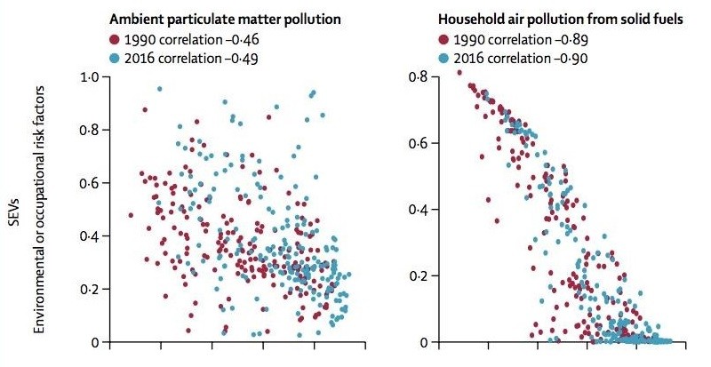
Figure 7. Relationship between Summary Exposure Values (SEVs, y-axis) and Socio-demographic Index (SDI, x-axis) for the three environmental risk factors that are responsible for the largest number of attributable DALYs globally. 64Figure source: Global Burden of Disease (GBD). (14 Sept 2017). 2016 Risk Factors Collaborators. Global, regional, and national comparative risk assessment of 84 behavioural, environmental and occupational, and metabolic risks or clusters of risks, 1990–2016: a systematic analysis for the Global Burden of Disease Study 2016. The Lancet, 390: 1345-1422. SEV is a metric that captures the risk-weighted exposure or prevalence of an exposure for a population. SEV values range from 0% (no risk exposure in a population) to 100% (the entire population is exposure to the maximum possible level for that risk). SDI is a summary measure of a region’s socio-demographic development based on average income per person, educational attainment, and total fertility rate. SDI values range from 0 (lowest income per capita, lowest educational attainment, and highest total fertility rate) to 1 (the highest income per capita, highest educational attainment, and lowest total fertility rate). The graphs illustrate that summary exposure values to both household air pollution from solid fuels and ambient particulate air pollution are larger for populations with lower SDI values.
C O N T E N T S